Excess deaths due to COVID-19

import pandas as pd
from pymc_extras.prior import Prior

import causalpy as cp

OMP: Info #276: omp_set_nested routine deprecated, please use omp_set_max_active_levels instead.

%load_ext autoreload
%autoreload 2
%config InlineBackend.figure_format = 'retina'
seed = 42

Load data

df = (
    cp.load_data("covid")
    .assign(date=lambda x: pd.to_datetime(x["date"]))
    .set_index("date")
)

treatment_time = pd.to_datetime("2020-01-01")
df.head()

	temp	deaths	year	month	t	pre
date
2006-01-01	3.8	49124	2006	1	0	True
2006-02-01	3.4	42664	2006	2	1	True
2006-03-01	3.9	49207	2006	3	2	True
2006-04-01	7.4	40645	2006	4	3	True
2006-05-01	10.7	42425	2006	5	4	True

The columns are:

• date + year: self explanatory

• month: month, numerically encoded. Needs to be treated as a categorical variable

• temp: average UK temperature (Celsius)

• t: time

• pre: boolean flag indicating pre or post intervention

Run the analysis

In this example we are going to standardize the data. So we have to be careful in how we interpret the inferred regression coefficients, and the posterior predictions will be in this standardized space.

First, we’ll build a linear regression model, but specify custom priors for the regression coefficients beta and the likelihood distribution y_hat. We stick with a relatively simple specification for the mu values of the coefficients, sticking with zero for all but the intercept. A value of 42,000 was chosen as this is the approximate median number of deaths per month in the UK.

model = cp.pymc_models.LinearRegression(
    sample_kwargs={"random_seed": seed},
    priors={
        "beta": Prior(
            "Normal",
            mu=[42_000, 0, 0, 0, 0, 0, 0, 0, 0, 0, 0, 0, 0, 0],
            sigma=10_000,
            dims=["treated_units", "coeffs"],
        ),
        "y_hat": Prior(
            "Normal",
            sigma=Prior("HalfNormal", sigma=10_000, dims=["treated_units"]),
            dims=["obs_ind", "treated_units"],
        ),
    },
)

Now we’ll build the InterruptedTimeSeries experiment object, passing in our custom model. The formula specifies:

• an intercept term (1)

• a linear trend over time (t)

• a categorical variable for month (month)

• a temperature variable (temp)

result = cp.InterruptedTimeSeries(
    df,
    treatment_time,
    formula="deaths ~ 1 + t + C(month) + temp",
    model=model,
)

Initializing NUTS using jitter+adapt_diag...
Multiprocess sampling (4 chains in 4 jobs)
NUTS: [beta, y_hat_sigma]

Sampling 4 chains for 1_000 tune and 1_000 draw iterations (4_000 + 4_000 draws total) took 3 seconds.
Sampling: [beta, y_hat, y_hat_sigma]
Sampling: [y_hat]
Sampling: [y_hat]
Sampling: [y_hat]
Sampling: [y_hat]

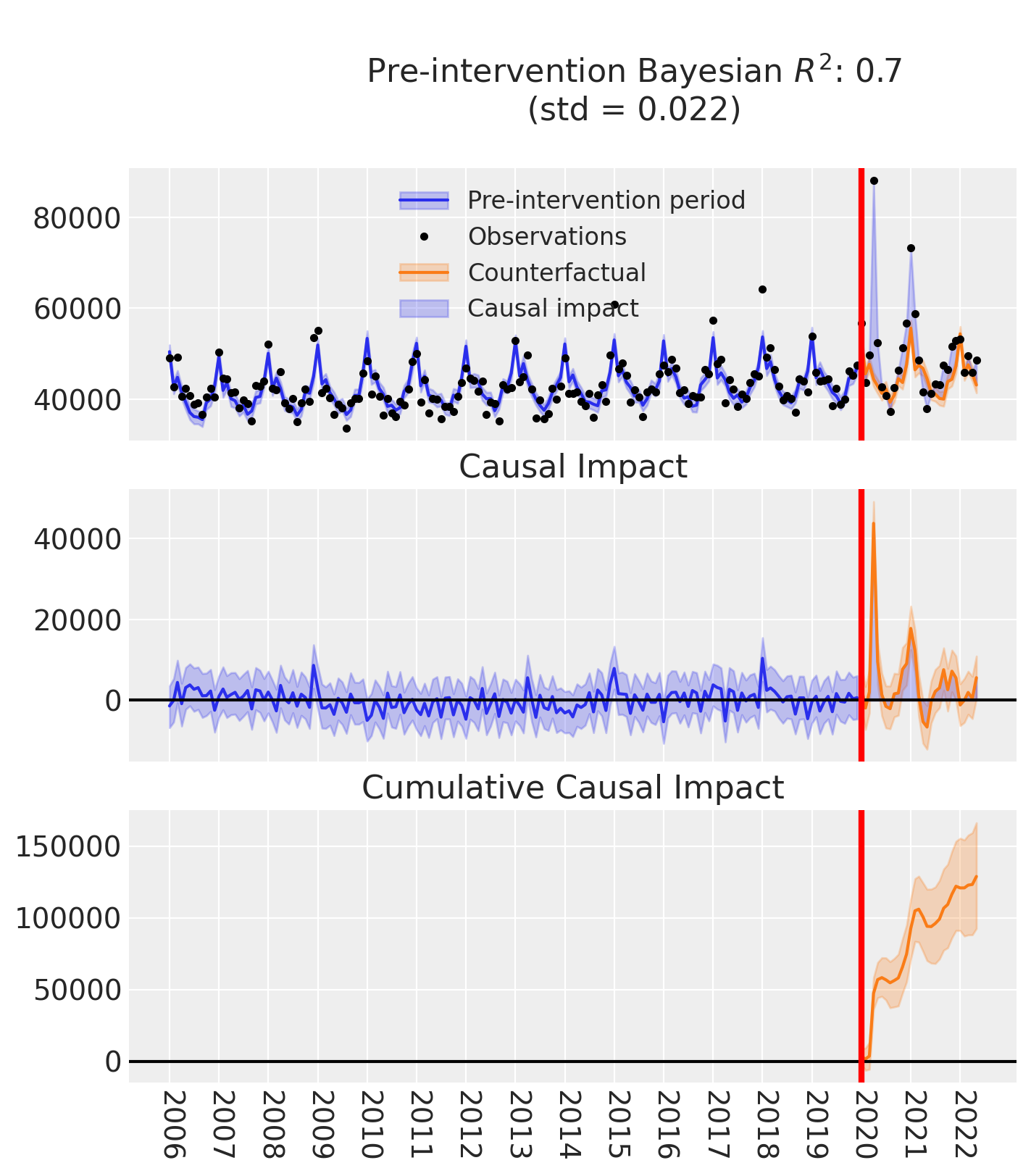
fig, ax = result.plot()

# figure customization
ax[2].set_xticks(pd.date_range(start=df.index.min(), end=df.index.max(), freq="YS"))
ax[2].set_xticklabels(
    pd.date_range(start=df.index.min(), end=df.index.max(), freq="YS").year
)
ax[2].tick_params(axis="x", rotation=-90)

result.summary()

==================================Pre-Post Fit==================================
Formula: deaths ~ 1 + t + C(month) + temp
Model coefficients:
    Intercept       52799, 94% HDI [50959, 54693]
    C(month)[T.2]   -8029, 94% HDI [-9934, -6187]
    C(month)[T.3]   -5622, 94% HDI [-7518, -3698]
    C(month)[T.4]   -6761, 94% HDI [-8901, -4585]
    C(month)[T.5]   -6953, 94% HDI [-9777, -4217]
    C(month)[T.6]   -6890, 94% HDI [-10198, -3573]
    C(month)[T.7]   -5737, 94% HDI [-9579, -1946]
    C(month)[T.8]   -7716, 94% HDI [-11411, -4157]
    C(month)[T.9]   -8068, 94% HDI [-11350, -4873]
    C(month)[T.10]  -6600, 94% HDI [-9115, -4114]
    C(month)[T.11]  -8520, 94% HDI [-10485, -6526]
    C(month)[T.12]  -6696, 94% HDI [-8618, -4820]
    t               23, 94% HDI [16, 31]
    temp            -621, 94% HDI [-921, -331]
    y_hat_sigma     2684, 94% HDI [2421, 3001]